Python编程
计算并打印出从 1 到 10 的所有偶数
程序
for i in range(1, 11):
    if i % 2 == 0:
        print(i)
输出
2
4
6
8
10

Process finished with exit code 0
接受用户输入的两个数字,并计算它们的和
程序
print("Please enter the first number:")
a = int(input())
print("Please enter the second number:")
b = int(input())
c = a + b
print("The sum of the two numbers is", c)
输出
Please enter the first number:
10
Please enter the second number:
20
The sum of the two numbers is 30

Process finished with exit code 0
找出给定列表中的最大值和最小值,并打印它们
程序
# Define a list of numbers
numbers = [4, 2, 9, 7, 5, 1, 8, 3, 6]

# Print the list
print("List of numbers: ", numbers)

# Find the maximum and minimum value
max_value = max(numbers)
min_value = min(numbers)

print("Maximum: ", max_value)
print("Minimum:", min_value)
输出
List of numbers:  [4, 2, 9, 7, 5, 1, 8, 3, 6]
Maximum:  9
Minimum: 1

Process finished with exit code 0
接受用户输入的一个字符串,并判断该字符串是否为回文字符串
程序
def is_palindrome(s):
    return s == s[::-1]


# 测试代码
string = input("Please input a string:")
if is_palindrome(string):
    print("This is a palindrome string.")
else:
    print("This is not a palindrome string.")
输出
List of numbers:  [4, 2, 9, 7, 5, 1, 8, 3, 6]
Maximum:  9
Minimum: 1

Process finished with exit code 0
生成斐波那契数列的前 n 个数字,其中 n 是用户输入的一个整数
程序
def fibonacci(n):
    fib_sequence = [0, 1]
    while len(fib_sequence) < n:
        fib_sequence.append(fib_sequence[-1] + fib_sequence[-2])
    return fib_sequence[:n]


number = int(input("Please input a number:"))
print(fibonacci(number))
输出
Please input a number:10
[0, 1, 1, 2, 3, 5, 8, 13, 21, 34]

Process finished with exit code 0
软件包管理
本地计算机(macOS Sonoma操作系统)上采用miniconda和mamba forge进行软件包的管理工作,已经将所有包管理软件的软件源切换成国内的清华源以加快访问速度。
完成任务的bash脚本如下:
#! /bin/zsh
pip update
pip install numpy
pip upgrade pandas
pip install matplotlib
conda create myenv
conda activate myenv
mamba install numpy
mamba install pandas
conda list --export > requirements.txt
输出的列出了该conda环境中已安装的所有软件包的requirements.txt文件为:
# This file may be used to create an environment using:
# $ conda create --name <env> --file <this file>
# platform: osx-arm64
blas=1.0=openblas
bottleneck=1.3.7=py311hb9f6ed7_0
brotli=1.0.9=h80987f9_8
brotli-bin=1.0.9=h80987f9_8
bzip2=1.0.8=h80987f9_6
ca-certificates=2024.3.11=hca03da5_0
contourpy=1.2.0=py311h48ca7d4_0
cycler=0.11.0=pyhd3eb1b0_0
fonttools=4.51.0=py311h80987f9_0
freetype=2.12.1=h1192e45_0
jpeg=9e=h80987f9_1
kiwisolver=1.4.4=py311h313beb8_0
lcms2=2.12=hba8e193_0
lerc=3.0=hc377ac9_0
libbrotlicommon=1.0.9=h80987f9_8
libbrotlidec=1.0.9=h80987f9_8
libbrotlienc=1.0.9=h80987f9_8
libcxx=14.0.6=h848a8c0_0
libdeflate=1.17=h80987f9_1
libffi=3.4.4=hca03da5_1
libgfortran=5.0.0=11_3_0_hca03da5_28
libgfortran5=11.3.0=h009349e_28
libopenblas=0.3.21=h269037a_0
libpng=1.6.39=h80987f9_0
libtiff=4.5.1=h313beb8_0
libwebp-base=1.3.2=h80987f9_0
llvm-openmp=14.0.6=hc6e5704_0
lz4-c=1.9.4=h313beb8_1
matplotlib=3.8.4=py311hca03da5_0
matplotlib-base=3.8.4=py311h7aedaa7_0
ncurses=6.4=h313beb8_0
numexpr=2.8.7=py311h6dc990b_0
numpy=1.26.4=py311he598dae_0
numpy-base=1.26.4=py311hfbfe69c_0
openjpeg=2.3.0=h7a6adac_2
openssl=3.0.13=h1a28f6b_1
packaging=23.2=py311hca03da5_0
pandas=2.2.1=py311h7aedaa7_0
pillow=10.3.0=py311h80987f9_0
pip=24.0=py311hca03da5_0
pyparsing=3.0.9=py311hca03da5_0
python=3.11.9=hb885b13_0
python-dateutil=2.9.0post0=py311hca03da5_0
python-tzdata=2023.3=pyhd3eb1b0_0
pytz=2024.1=py311hca03da5_0
readline=8.2=h1a28f6b_0
setuptools=69.5.1=py311hca03da5_0
six=1.16.0=pyhd3eb1b0_1
sqlite=3.45.3=h80987f9_0
tk=8.6.14=h6ba3021_0
tornado=6.3.3=py311h80987f9_0
tzdata=2024a=h04d1e81_0
unicodedata2=15.1.0=py311h80987f9_0
wheel=0.43.0=py311hca03da5_0
xz=5.4.6=h80987f9_1
zlib=1.2.13=h18a0788_1
zstd=1.5.5=hd90d995_2
生物信息分析
依赖安装及环境配置
需要引用的包有:
import matplotlib.pyplot as plt
import numpy as np
import pandas as pd
from scipy import stats
import seaborn as sns
数据集下载
由于磁盘空间限制,我采用的是题目示例1中的GSE5583数据集,可以从https://www.ncbi.nlm.nih.gov/geo/query/acc.cgi?acc=GSE5583底部的FTP站点进行下载。
进行分析
载入数据
# Load the data
data = pd.read_table('./data/GSE5583_series_matrix.txt', skiprows=67, header=1, index_col=0)
可通过head()查看数据的头几行如下:
The first few rows of the data are:
           GSM130365  GSM130366  GSM130367  GSM130368  GSM130369  GSM130370
ID_REF
100001_at       11.5        5.6       69.1       15.7       36.0       42.0
100002_at       20.5       32.4       93.3       31.8       14.4       22.9
100003_at       72.4       89.0       79.2       80.5      130.1       86.7
100004_at      261.0      226.2      365.1      432.0      447.3      288.1
100005_at     1086.2     1555.6     1487.1     1062.2     1365.9     1436.2
对数据进行预处理
采用取对数的方式对数据进行预处理:
data2 = np.log2(data+0.0001)
print("\nThe first few rows of the stabilized data are:")
print(data2.head())
预处理结果可通过head()进行部分输出:
The first few rows of the stabilized data are:
           GSM130365  GSM130366  GSM130367  GSM130368  GSM130369  GSM130370
ID_REF
100001_at   3.523575   2.485453   6.110616   3.972702   5.169929   5.392321
100002_at   4.357559   5.017926   6.543807   4.990959   3.848007   4.517282
100003_at   6.177920   6.475735   6.307430   6.330919   7.023478   6.437962
100004_at   8.027907   7.821456   8.512148   8.754888   8.805099   8.170426
100005_at  10.085074  10.603256  10.538286  10.052840  10.415636  10.488041
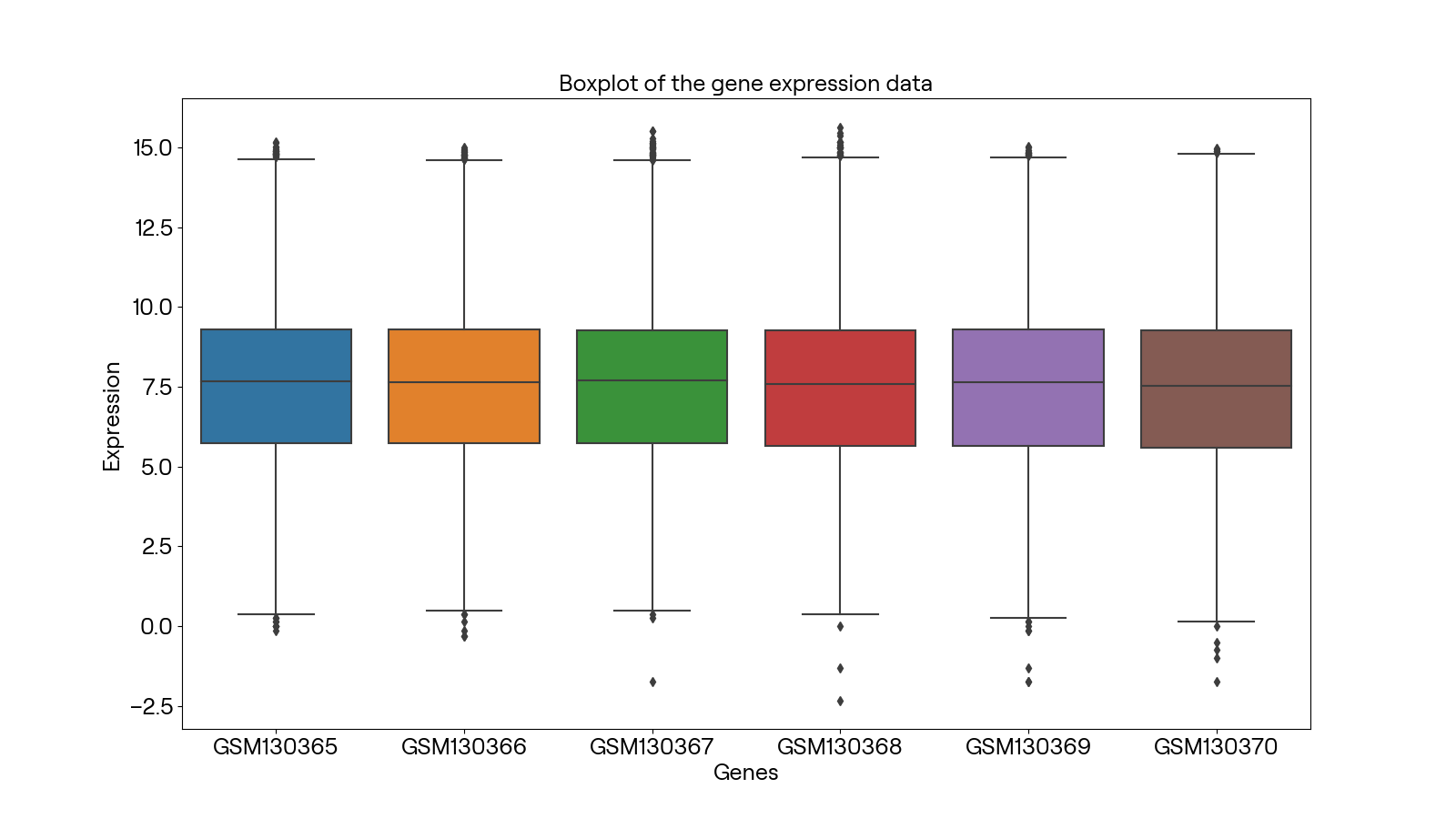
同时利用matplotlib及seaborn库画出每个阵列的箱线图如下:
为查看不同样本之间是否有总体差异,我们再画出每个基因表达量的密度分布图:
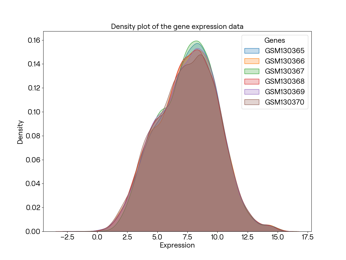
可以看出样本之间基本没有总体差异,可以做差异分析。
差异分析
计算每个基因wt及ko样本的表达平均值
# Calculate the mean of the WT samples
wt = data2.loc[:, 'GSM130365' : 'GSM130367'].mean(axis = 1)

# Calculate the mean of the KO samples
ko = data2.loc[:,'GSM130368':'GSM130370'].mean(axis = 1)
同理,可通过head()函数进行前几行的输出:
The first few rows of the mean of the WT samples are:
ID_REF
100001_at     4.039881
100002_at     5.306431
100003_at     6.320362
100004_at     8.120504
100005_at    10.408872
dtype: float64

The first few rows of the mean of the KO samples are:
ID_REF
100001_at     4.844984
100002_at     4.452083
100003_at     6.597453
100004_at     8.576804
100005_at    10.318839
dtype: float64
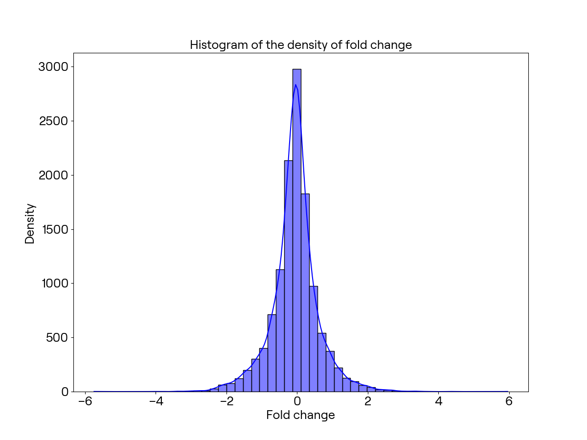
令fold为这两个样本表达平均值的差,我们可以制作出直方图如下:
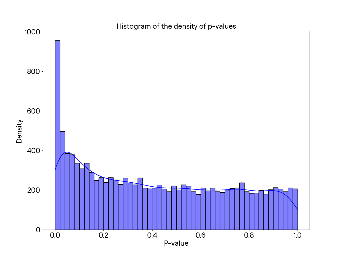
p-value差异化分析
随后进行基因样本的T-检验及p值计算:
# Calculate the t-statistic and p-value
pvalue = []
number_of_genes = data2.shape[0]
for i in range(0, number_of_genes):
    ttest = stats.ttest_ind(data2.iloc[i,0:3], data2.iloc[i,3:6])
    pvalue.append(ttest[1])
使用head()查看结果:
The first few p-values are:
[0.5273743930676532, 0.30530698472095097, 0.2980791701563722, 0.18923599966356336, 0.6921016401581233]
生成图表